경제 뉴스에서 자주 등장하는 용어 중 하나가 바로 “경제성장률”이다.

뉴스에서는 “이번 분기 경제성장률이 전년 동기 대비 2.2% 증가했다” 또는 “전기 대비 0.6% 성장”과 같은 문장을 어렵지 않게 접할 수 있다. 하지만 이 숫자들이 정확히 무엇을 뜻하는지, 또 어떤 기준으로 측정되는지 궁금했던 적은 없었을까?

경제성장률은 말 그대로 국가 경제가 얼마나 커졌는지를 나타내는 비율이다. 일반적으로 GDP(국내총생산)의 증감률을 통해 측정한다.

📌 GDP란 무엇일까?

GDP는 Gross Domestic Product의 줄임말로, 일정 기간 동안 한 나라 안에서 새로 생산된 재화와 서비스의 총합을 뜻한다. 쉽게 말해, 한 나라가 얼마만큼의 ‘경제 활동’을 했는지를 돈으로 환산한 것이다.

예를 들어, 사람들이 커피를 사고, 치킨을 먹고, 회사가 자동차를 만들고, 집을 짓는 모든 행위가 GDP에 포함된다.

📌 실질 GDP vs 명목 GDP

경제성장률을 정확히 보기 위해선 실질 GDP를 사용해야 한다.

왜냐하면 명목 GDP는 물가 상승(인플레이션)의 영향을 그대로 반영하기 때문에, 실제로 생산된 양이 늘었는지, 아니면 단지 가격이 오른 건지 알 수 없기 때문이다.

실질 GDP는 물가 상승분을 제거한 값으로, 진짜로 경제가 성장했는지를 보여주는 지표다.

🌿 덧붙임: 계절조정 GDP란?

경제는 우리가 숨 쉬는 일상처럼 계절에 따라 반복되는 패턴을 가지고 있다.

예를 들어, 설날이나 추석 같은 명절 시즌에는 소비가 일시적으로 급증하고,

겨울철에는 난방용 에너지 소비가 늘고, 봄에는 농업 생산이 본격화된다.

이처럼 자연스럽게 반복되는 계절 요인은 GDP의 변동에도 영향을 미친다.

그런데 우리가 알고 싶은 건 ‘겨울이라 그런 것’이 아니라

진짜로 경제가 좋아진 건지, 혹은 나빠진 건지다.

그래서 등장한 것이 바로 계절조정 GDP이다.

즉, 계절조정 GDP는 계절의 영향(반복적인 요인)을 제거하고,순수한 경기 흐름만 파악할 수 있도록 만든 지표다.

📊 우리나라는 어떻게 활용하고 있을까?

우리나라에서는 통계청과 한국은행이 매 분기마다 실질 GDP와 그에 대한 계절조정값을 발표한다.

특히 전기비 성장률을 볼 때는 항상 계절조정된 실질 GDP를 사용한다.

왜냐하면 전기(1분기 → 2분기) 사이의 비교는 계절 차이를 반영하지 않으면 의미가 왜곡되기 때문이다.

예를 들어 1분기에는 설날이 있고, 2분기에는 없다고 치자.

만약 계절조정을 하지 않고 그냥 비교하면 1분기의 소비는 더 높게 나올 수밖에 없다.

하지만 이는 실제 경기 상황이 좋아서가 아니라 설날 특수 때문일 수 있다.

이런 왜곡을 없애고자 계절조정된 GDP를 통해 “실질적인 경기 변화”를 파악하는 것이다.

📌 전년동기비? 전기비?

경제성장률은 보통 두 가지 방식으로 표현된다.

• 전년동기비(전년 동기 대비):→ 계절의 영향을 제거하고 전체적인 경기 흐름을 볼 때 유용하다.
• 작년 같은 시기(예: 작년 1분기)와 비교한 성장률.
• 전기비(전 분기 대비):→ 경제의 단기적인 변화나 속도를 파악할 때 유용하다.
• 예를 들어, 전기비 성장률이 계속 마이너스라면 경기 침체의 조짐일 수 있다.
• 바로 직전 분기(예: 올해 1분기와 2분기)를 비교한 성장률.

📌 성장기여도란?

여기서 한 걸음 더 나아가면 “성장기여도”라는 개념이 등장한다.

이는 경제성장률에 어떤 분야가 얼마나 기여했는지를 보여주는 지표다.

예를 들어, 전체 성장률이 2%인데 민간소비가 1.2%, 수출이 0.8%를 기여했다면, 이 두 항목이 경제성장을 견인했다는 뜻이다.

반대로 정부지출이나 설비투자가 성장기여도가 -로 나타난다면, 이 분야가 오히려 성장률을 낮추는 요인으로 작용한 것이다.

따라서 성장기여도를 보면 단순히 “얼마나 성장했는가”를 넘어서 “누가 성장하게 만들었는가”까지 알 수 있다.

어떤 지표가 중요할까?

불확실성이 큰 요즘에는 단순한 성장률보다는 질적인 성장, 그리고 누가 기여하고 있는지를 보여주는 성장기여도 분석이 중요해지고 있다. 또한 소비와 수출이 어느 쪽에서 탄력을 받고 있는지를 따지는 것도 기업이나 투자자에겐 매우 중요한 참고자료가 된다.

음식점에서 음식을 파는 방법도 경제 상황에 따라 다양하다. 예를 들어 경제가 호황인 시기에는 사람들의 소비가 활발히 이루어지므로 치킨 두 마리 세트를 팔지만 요즘 같은 경제 불황 시기에는 치킨 반 마리만 판매하기도 한다.

이처럼 전체적인 경기의 수준이 주기적으로 상승, 하강하는 현상을 경기변동 이라고 한다. 경기변동은 호황, 후퇴, 불황, 회복기의 총 4단계로 나뉜다. 이러한 단계 속에서 경제 상황을 판단하는 것이 꽤 중요하다고 할 수 있다.

경기종합지수란 앞으로 경제 상황이 어떻게 될지 예측하거나, 현재 경제 상황을 판단하는 데 사용하는 주요 지표 중 하나이며 정확히는 생산, 소비, 고용, 금융, 무역, 투자 등 경제 부문의 지표를 종합한 지수를 의미하며 크게 세 가지로 나뉜다.

첫번째는 선행종합지수로 앞으로의 경제 상황을 예측할 때 사용하는 지표이며, 경제심리지수 & 건설수주액수 등이 포함된다. 다양한 기업과 은행들은 이 지표를 참고하여 앞으로의 경제상황을 예측하고 사전에 대비한다.

두번째는 동행종합지수로 현재 경제상황을 보여주는 지표이다. 광공업생산지수 및 소매판매액지수 등이 이에 포함된다.

마지막은 후행종합지수로 경제를 예측 후 사후에 예측과 실제 경제 변동의 차이를 확인하는 지표이다 (과거의 경제 상태를 나타낸다). 소비재수입액, 기업어음유통수익률 등이 이에 포함된다.

각 상황을 반영한 새로운 지표를 만든다면 무엇이 있을까?

참고: https://youtu.be/YqdxeAzPajg?si=MlTFy6gdgZG3dCUk

0. Introduction

Point process model 혹은 exponential random graph model (ergm) 등과 같은 통계적 모형은 bayesian inference가 쉽지 않다. 그 이유는 지난 [Speeding up MCMC by Delayed Acceptance and Data Subsampling] 논문에서 밝힌 바와 비슷하게, 아래와 같이 function의 normalizing constant($z(\boldsymbol \theta)$)가 parameter의 function이기 때문에 likelihood($L(\boldsymbol \theta | \mathbf x) = h(\mathbf x | \boldsymbol \theta) / z(\boldsymbol \theta)$)를 구하는 것이 computational expensive 하기 때문이다. (Posterior distribution은 다음과 같이 쓸 수 있다)

$$\pi(\boldsymbol \theta | \mathbf x) \propto p(\boldsymbol \theta) \frac{h(\mathbf x| \boldsymbol \theta)}{z(\boldsymbol \theta)} $$

위 문제를 해결하기 위한 여러 방법 중 가장 널리 쓰이는 방법은 auxiliary variable을 generate하여 likelihood의 normalizing constant 부분을 cancel out하는 double metropolis hastings (DMH) 알고리즘, 혹은 likelihood를 구하지 않고 proposed된 parameter하에서 sample을 생성하여 이것을 accept or reject하는 likelihood-free 알고리즘인 approximate bayesian computation(ABC) 알고리즘 등이 있다.

하지만 여전히 두 알고리즘 역시 theoretical한 측면에서 guarantee 되거나 computational expensive하다는 장점이 있다. 따라서 이 논문에서 저자들은 likelihood function의 normalizing constant를 Gaussian process approximation을 통하여 approximate하는 새로운 알고리즘을 제시한다.

1. Function Emulation

논문에서 중요한 개념 중 하나인 function emulation이란 함수를 계산하는 것이 어려울 때 approximate한 함수를 사용하는 방법이다. 예를 들어 위의 likelihood function의 normalizing constant $z(\boldsymbol \theta)$를 계산하는 것이 어렵다면 이 부분을 approximate하여 likelihood 계산에 사용하는 것이다.

이 방법은 point process model 혹은 ergm 과 같이 likelihood 계산이 복잡한 문제에 대해서 기존의 DMH 등의 알고리즘보다 bayesian inference를 computationally effcient하게 할 수 있다는 것이 장점이다. 저자들이 제시한 알고리즘은 다음과 같이 크게 두 단계로 구성된다.

(1) normalizing constant을 importance sampling을 사용하여 approximate

(2) Gaussian process를 사용하여 관측되지 않은 parameter의 importance sampling estimate

2. Algorithm

p-dimensional parameter $\boldsymbol \theta \in \Theta$에 대하여, $\Theta$안의 $d$개의 particle, $\psi = (\boldsymbol \theta^{(1)}, \dots,\boldsymbol \theta^{(d)})$, 을 고려해보자. 그리고 $\tilde{\boldsymbol \theta}$를 MPLE or sample mean 등의 mle의 approximation 값이라고 하자.

그렇다면 우리는 $(Z(\boldsymbol\theta^{(1)})/Z(\tilde{\boldsymbol\theta}),\dots,Z(\boldsymbol\theta^{(d)})/Z(\tilde{\boldsymbol \theta}))$의 unbiased Monte Carlo estimate를 importance sampling을 사용하여 아래와 같이 log scale로 estimate 할 수 있다 (이것의 estimate가 필요한 이유는 MCMC algorithm으로 acceptance probability를 계산할 때 해당 부분을 계산해야 하는데, 이것이 어렵기 때문에 위의 MC estimate를 사용하는 것이다).

$$ \log \widehat Z_{IS}(\boldsymbol\theta^{(i)}) = \log\Big( \frac{1}{N} \sum_{l=1}^N \frac{h(\mathbf x_l | \boldsymbol \theta^{(i)})}{h(\mathbf x_l | \tilde{\boldsymbol \theta})}\Big)$$

각 $\mathbf x_l$은 l-th Markov chain의 마지막 샘플을 의미한다. 위의 MC estimate를 각 d개의 particle에 대하여 모두 모은 것을 $\log \hat{\mathbf Z}_{IS} = (\log \hat{Z}_{IS}(\boldsymbol\theta^{(1)}),\dots,\log \hat{Z}_{IS}(\boldsymbol\theta^{(d)}))^\prime \in \mathbb R^d$ 라고 하자. 우리는 아래와 같이 Gaussian process model을 정의할 수 있다.  ($\boldsymbol \mu$ is the mean and $\mathbf u$ is a second-order stationary Gaussian process)

$$\log\hat{\mathbf Z}_{IS} = \boldsymbol \mu + \mathbf u$$

또한 새로운 parameter $\boldsymbol \theta^* \in \Theta$에 대하여, 우리는 Gaussian process의 definition을 사용하여 아래와 같은 multivariate gaussian normal model을 정의할 수 있다. (simple linear mean trend $\boldsymbol \mu = \boldsymbol \psi \boldsymbol \beta$를 가정, $\mathbf C$ and $\mathbf c$ are the covariance functions in equation (4) in the paper, and $\tau^2 \ \& \ \sigma^2$ are the parameters of covariance function)

$$\begin{align*}\begin{bmatrix} \log \hat{\mathbf Z}_{IS}\\ \log \hat{Z}_{IS}(\boldsymbol \theta^*)\end{bmatrix} &\sim \text{MVN}\begin{pmatrix} \begin{bmatrix} \boldsymbol \psi \boldsymbol\beta \\ \boldsymbol \theta^* \boldsymbol \beta \end{bmatrix}\! ,& \begin{bmatrix} \mathbf C & \mathbf c \\ \mathbf c^\prime & \sigma^2 + \tau^2 \end{bmatrix}\end{pmatrix} \end{align*}$$

따라서 우리는 새로운 $\theta^*$의 likelihood를 매번 계산하지 않고, 주어진 $d$개의 particle set을 사용하여 만든 위 Gaussian process approximation을 통하여 $\log \hat Z(\boldsymbol \theta^*) | \log \hat{\mathbf Z}_{IS}$를 구할 수 있고, 이것을 사용하여 best linear unbiased predictor(BLUP)를 구할 수 있다. (논문 equation (6) ~ (8) 참고)

논문의 알고리즘 1을 살펴보면, Part 1에서는 위 과정 중 importance sampling approximation 부분을 수행하며, Part 2에서는 Part 1에서 만든 importance sampling approximation을 사용해 새롭게 propose되는 theta에 대한 Gaussian process approximation을 수행하여 likelihood를 우회적으로 계산 후 acceptance probability를 계산해 sample의 accept 여부를 결정한다.

또한 likelihood의 normalizing constant part가 intractable한 상황이 아니라 likelihood의 계산 자체가 intractable한 경우 역시 likelihood function 자체를 emulation 하는 방법을 통해 논문의 알고리즘 2와 같이 극복할 수 있다.

다른 중요한 한가지는 d 개의 parameter에 대한 particle을 만들 때, 각 particle이 parameter space의 중요한 부분을 잘 cover하도록 만드는 것이다. 저자들은 DMH or ABC algorithm을 사용하면 효과적으로 중요한 parameter space를 cover하는 particle을 만들 수 있음을 알고리즘 3, 4를 통하여 밝힌다.

3. Application

마지막으로 저자들이 만든 알고리즘을 기존의 DMH와 비교한 real data application 실험을 진행하였다. 실험은 총 두 가지로 첫번째는  실제 social network data와 simulated data를 ergm을 사용하여 fitting한 모델의 parameter를 estimate한 결과와 computation time을 비교한 실험이며, 두번째는 attraction-repulsion point process 모델의 Parameter 추정 및 computation 시간을 비교한 것이다.

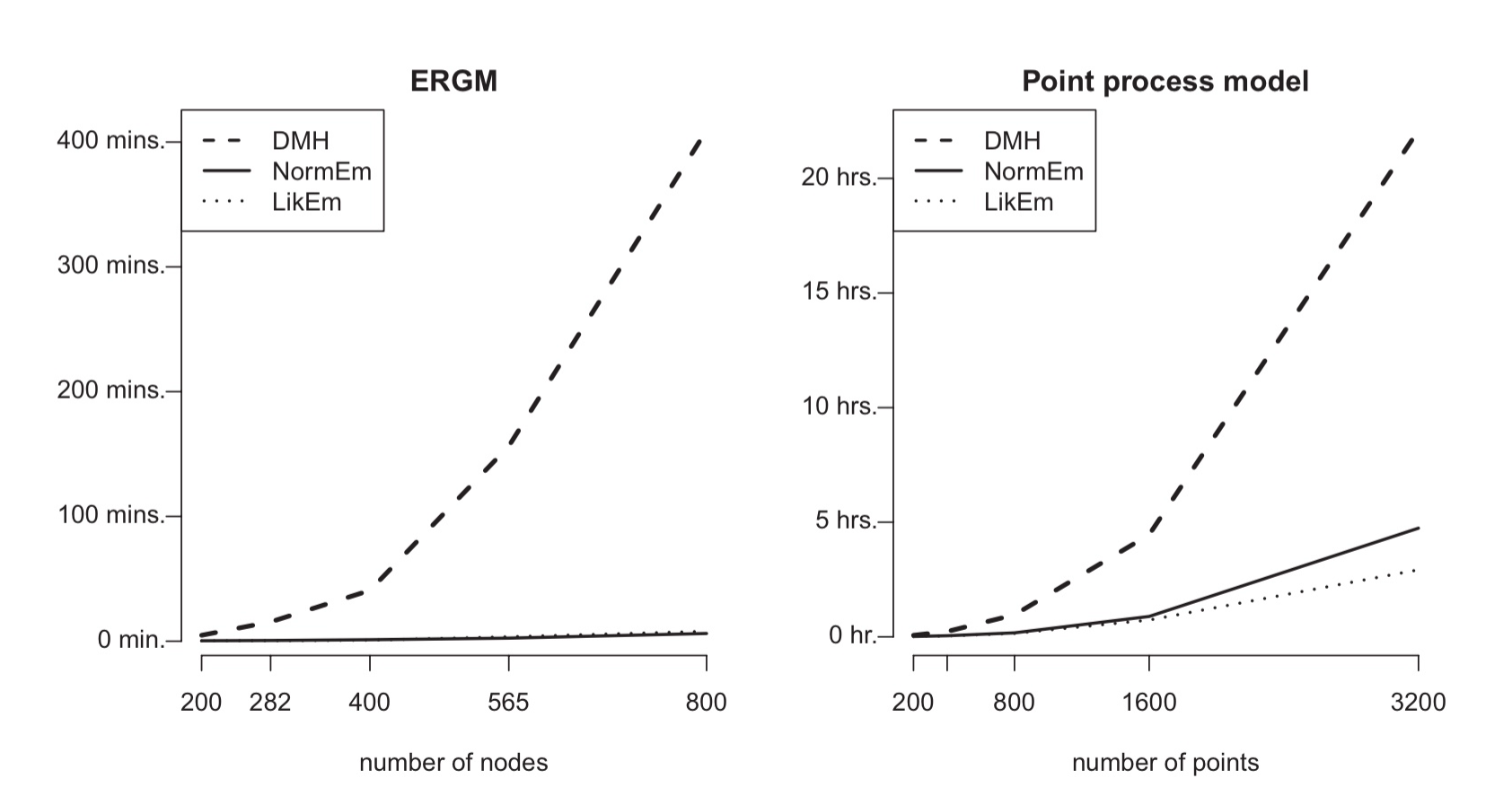
중요한 비교 결과는 두 실험 모두에서 DMH 알고리즘에 비해 크게 computation time을 단축시켰다는 것이다. 아래에 첨부한 Figure 1을 보면 큰 데이터 셋에 대하여 computing 시간이 DMH에 비교해 훨씬 줄어든 것을 확인할 수 있으며, parameter estimation 결과는 비슷한 것을 확인할 수 있다.

Reference:

Park, J., & Haran, M. (2020). A function emulation approach for doubly intractable distributions. Journal of Computational and Graphical Statistics, 29(1), 66-77.

Link:

https://www.tandfonline.com/doi/full/10.1080/10618600.2019.1629941?casa_token=XKpfYl743TUAAAAA%3AfFdKaRxkgDgl68nTbjn0QvRtI1ExBBrtobCw_eb707hZwVwM1Pr1m2cCAJMg7X0OVimOndrthvTExw

0. Introduction

대부분의 MH algorithm은 단순한 모델에서는 적용이 잘 되지만, full data가 너무 크거나 intractable한 constant term을 포함하고 있어 이것의 likelihood를 얻기 어려운 경우는 적용이 어렵다는 단점이 있다. 예를 들어 Ising model과 같이 intractable constant를 포함한 모델에서 full data를 사용하여 likelihood를 계산하는데 필요한 computation이 grid 수가 증가함에 따라 2의 제곱배로 늘어난다.

따라서 이를 극복하기 위해 다양한 MH 알고리즘이 개발되어 왔다. Double Metropolis Hastings (DMH)나 Approximate Bayesian Computation (ABC)도 그것의 예시들이다. 이 논문에서 다루는 알고리즘은 Delayed Acceptance MH (DAMH) 알고리즘으로, 간단히 말하자면 두 단계로 나누어서 sample의 accept / reject 를 결정하는 알고리즘이다. 첫번째 단계에서는 random subsample을 기반으로 likelihood function을 approximate하여 잠재적인 sample의 accept 여부를 결정한다. 이 단계에서 accept된 sample에 한하여 두번째 단계로 넘어가게 되는데, 두번째 단계에서는 full data의 likelihood를 계산하여 최종적인 sample의 수락 여부를 결정한다.

이렇게 되면 sample을 propose한 후 매번 full data의 likelihood를 계산할 필요 없이, accept될 가능성이 보이는 sample에 대해서만 likelihood of full data를 계산하면 되기 때문에 기존의 MH 알고리즘보다 computation 측면에서 더욱 효율적이다.

하지만 앞서 말했듯 full data의 likelihood를 계산하는 자체가 불가능하거나 어려운 경우가 많다. 따라서 이들은 subsample을 사용한 likelihood의 estimation 방법을 제안하여 DAMH의 기존 어려움을 해결하고자 하였으며 이들의 방법이 기존의 DAMH 방법보다 더욱 효율적이고 계산 속도를 높일 수 있음을 보였다.

1. Likelihood estimator

k-th observation의 log density의 notation은 다음과 같으며 아래에서 $(y_k, x_k, \theta)$는 각각 k-th response, covariates, and model parameter를 의미하며 data size는 총 $n$개이다.

$$l_k(\theta) = \log p(y_k | \theta, x_k)$$

또한 위의 log density를 사용하여 다음과 같이 likelihood function을 정의하며, $l(\theta) = \sum_{k=1}^n l_k(\theta)$는 full data의 likelihood function을 나타낸다.

$$p(y|\theta) = \exp [l(\theta)]$$

위의 likelihood function을 estimate하기 위하여 size $m$의 sample을 사용한다. 하지만 Simple random sampling (SRS) 방법을 사용하여 sampling을 하기 보다는 이들은 control variates 방법을 활용하여 sampling을 수행한다. 먼저 다음과 같이 log likelihood를 decompose 한다.

$$\begin{align} l(\theta) & = \sum_{k=1}^n q_k(\theta) + \sum_{k=1}^n [l_k(\theta) - q_k(\theta)] \\ & = q(\theta) + d(\theta) \end{align}$$

그리고 위 식의 $d(\theta) = d$ term을 estimate하는 것을 목표로 하며 최종적으로 log likelihood를 $\hat l_m = \sum_{k=1}^n q_k (\theta) + \hat d_m$와 같이 estimate 한다.

($l, q$의 차이로 $d$를 계산할 수 있다. 그리고 이것을 활용하여 $\eta_i$를 정의한다. $m$개 sampling한 eta의 sample mean을 통해 $\hat d_m$을 추정할 수 있으며, 최종적으로 이것을 활용하여 log likelihood를 estimate하는 것이다. 또한 $d$를 줄이면 $q$가 log likelihood에 approximate하게 되므로 make sense 하다.)

이는 결과적으로 서로 유사한 $(x_k, y_k)$ 데이터 셋은 유사한 $l_k(\theta)$값을 보이므로, 비슷한 데이터끼리 clustering하는 효과를 주며, $l_k(\theta)$의 second order Taylor expansion을 사용하여 구한 $q$는 각 cluster의 centroid 주변에 위치하게 된다. 그리고 위처럼 estimate한 log likelihood를 원래 scale로 변환하면 bias가 생기게 되어 이를 unbiased하게 만들기 위해 논문의 2.4 수식과 같이 약간의 term을 추가하여 다음과 같이 exponential scale로 변환한다 (call it as a bias-corrected estimator).

$$\hat p_m (y | \theta, u) = \exp\Big(\hat l_m(\theta) - \hat \sigma^2_\eta (\theta)/2m\Big)$$

2. Delayed acceptance MH

Delayed acceptance MH의 목표 역시 parameter $\theta$에 대한 posterior distribution $\pi(\theta) = p(y | \theta)p(\theta)/p(y)$로 부터 sampling을 하는 것이다. Payne and Mallick이 제안한 DAMH 알고리즘은 다음과 같다.

● Algorithm

1. First stage에서는 current parameter $\theta_c = \theta^{(j)}$와 첫번째 proposal distribution $q_1$로부터 $\theta^\prime \sim q_1(\theta | \theta_c)$을 propose하여 아래의 probability를 계산한다. 이 때 위에서 estimate한 likelihood function $\hat p$를 사용한다 (but without using control variates for $\hat l_m$).

$$\alpha_1(\theta_c \rightarrow \theta^\prime) = \text{min} \Big\{1, \frac{\hat p_m(y| \theta^\prime, u) p(\theta^\prime) / q_1(\theta^\prime | \theta_c)} {\hat p_m (y | \theta_c,u) p(\theta_c) / q_1(\theta_c | \theta^\prime)}\Big\}$$

2. 위의 First stage를 거친 후 $\theta_p$를 $\alpha_1(\theta_c, \theta^\prime)$의 확률로 $\theta^\prime$로 propose하고 또는 $1-\alpha_1(\theta_c, \theta^\prime)$의 확률로 $\theta_c$로 propose 한다. 그 이후 아래 확률을 계산하여 최종적으로 $\theta^{(j+1)}$를 update한다. (First stage에서 reject가 일어난 $\theta_p = \theta_c$인 경우 확률이 1이되므로 $\theta^{(j+1)} = \theta^{(j)}$가 된다.)

$$\alpha_2(\theta_c \rightarrow \theta_p) = \text{min} \Big\{1, \frac{p(y | \theta_p) p(\theta_p) / q_2(\theta_p | \theta_c)}{p(y| \theta_c) p(\theta_c) / q_2(\theta_c | \theta_p)} \Big\}$$

Stage 2의 proposal $q_2$는 spike and slab(first stage의 $\alpha_1$을 weight로 함) density로 설정 가능하며, Payne and Mallick이 사용한 위 알고리즘의 first stage에서 estimated likelihood $\hat p_m$은 current state와 independent하기 때문에 standard MH theory를 따른다. 이 방법은 independent함을 사용하여 theoretical 하게 true posterior로의 수렴의 증명이 더 쉽다는 장점이 있다. 만약 이를 $\hat p_m(y| \cdot,u) = \hat p^{(\theta_c)}_m(y | \cdot, u)$와 같이 state dependent하게 만든다면 standard MH theory를 적용할 수는 없지만 parameter의 posterior distribution $\pi(\theta)$에 converge한다는 것이 입증되어 좋은 측면이 있다. 따라서 저자들은 후에 delayed acceptance block PMMH 알고리즘에서 이를 활용한다.

또한 위 알고리즘은 이들이 사용한 control variates 방법을 사용하지 않았는데, 이로 인하여 sample의 variance가 커지게 되어 결과적으로 estimated likelihood $\hat p_m$에 악영향을 끼치게 된다고 주장한다. 저자는 만약 control variates를 사용하여 likelihood를 estimate한다면 bias correction 과정 없이도 likelihood를 더 잘 estimate한다고 주장한다.

● 알고리즘 성능 측정

알고리즘의 성능을 비교하기 위하여 첫번째는 statistical efficiency가 있다. 이는 estimation이 더 작은 variance를 가지면 더 효율적인 것으로 여겨지며 estimate가 true 분포에 얼마나 근접한지를 의미한다. 두번째는 computational efficiency가 있다. 이는 주어진 iteration 동안 얼마나 효과적인 sample을 만들어내는지를 의미한다.

기존의 MH에 비해 DAMH는 less statistically efficient하다. 그 이유는 추가적인 수락 확률을 계산해야하기 때문이다. 두 번 거르는 작업을 하기 때문에 DAMH는 MH에 비해 새로운 sample을 accept할 확률이 상대적으로 낮아지며 따라서 더 강한 autocorrelation을 가질 확률이 높아진다. 이들은 Theorem 1을 통해 두번째 stage에서의 accpetance probability가 $\sigma^2_R$에 따라 수치적으로 변하는 양상을 설명한다.

반면 statistical and computational efficiency의 균형적인 측면에서는 DAMH가 MH에 비해 뛰어나다. DAMH는 첫번째 stage를 통해 수락 확률이 낮은 sample은 거르기 때문에 computational efficiency가 조금 더 나은측면이 있으며 sample의 variance를 줄일 수록 statistical efficiency 역시 증가하기 때문이다. 구체적인 성능 측정 지표는 논문의 equation 3.7 ~ 3.9에 나와있다.

3. Real data application

저자들은 자신의 control variates를 사용한 방법과 Payne and Mallick이 제안한 방법을 real data application을 통해 비교하였다. 각 방법을 사용해 스웨덴 기업의 1991~2008년도 기간동안의 534,717개 데이터를 covariate으로 하여 파산 확률을 모델링하였다. 구체적으로 아래와 같은 logistic regression model을 사용하고 beta의 prior distribution으로는 multivariate Gaussian distribution을 사용하였다.

$$p(y_k | x_k,\beta) = \frac{\exp(x_k^\top \beta)}{1+\exp(x_k^\top\beta)}$$

각 알고리즘의 수행 결과로 Effective Draws (ED) $= \frac{N}{IF \times t}$를 계산하여 이것을 각각의 분자로 하고, standard MH의 ED를 분모로 하여 Relative ED (RED) 값을 비교해 성능을 측정하였다. 따라서 table의 RED가 높을수록 성능이 더 뛰어나다고 할 수 있다. 이들의 알고리즘을 사용한 결과인 Table 1 과 Payne and Mallick의 방법을 사용한 Table 2를 비교해보면 Table 1의 RED값이 더 높으며 특히 Payne and Mallick의 방법은 매우 적은 수의 subsample을 사용한 경우 성능이 좋지 않았다. Table 1의 결과를 보면 더 많은 수의 subsample을 사용하면 두번째 stage의 acceptance probability 또한 높아져 알고리즘이 더 효율적인 결과를 낸다는 것을 확인할 수있다.

Reference:

Quiroz, M., Tran, M. N., Villani, M., & Kohn, R. (2018). Speeding up MCMC by delayed acceptance and data subsampling. Journal of Computational and Graphical Statistics, 27(1), 12-22.

Link:https://www.tandfonline.com/doi/full/10.1080/10618600.2017.1307117

Rcpp 파일은 c++에서 코드를 짠 후, 그것을 R에서 불러와서 실행할 수 있다.

c++로 코드를 짜는 것의 장점은 실행시간을 줄일 수 있다는 것인데 이는 c++에서는 코드를 짤 때 complie과정을 미리 거치는 반면, R이나 python에서는 코드를 실행할 때마다 complie을 하기 때문이다 (대신 디버깅이 쉬운 장점).

또한 window 운영체제와는 달리 Mac OS에서 이를 실행하는 것이 조금 까다롭다. 따라서 설치 후 실행에 성공한 방법을 간략히 적어보도록 하자.

1. Xcode 설치

Appstore 혹은 cmd창에 아래와 같은 command를 입력하여 Xcode를 설치한다.

xcode-select --install

2. Homebrew 설치

openMP를 설치하기 위해 homebrew라는 것이 필요한데 역시 command에 아래의 명령어를 입력하여 설치할 수 있다.

/bin/bash -c "$(curl -fsSL https://raw.githubusercontent.com/Homebrew/install/HEAD/install.sh)"

3. GCC 설치

역시 아래의 명령어를 이용하여 GCC를 설치한다. 또한 그 아래의 명령어로 gcc의 버전을 확인할 수 있다.

brew install gcc
gcc-14 --version

4. R에서 Rcpp & RcppArmadillo 패키지 설치

다음은 R에서 Rcpp 및 RcppArmaddillo 패키지를 설치한다.

install.packages("Rcpp")
install.packages("RcppArmadillo")

5. Rcpp 코드 작성 및 OpenMP 설정

이 부분이 조금 까다롭기도 한데 Makevars라는 것에 들어가서 직접 환경설정을 몇가지 해야 한다. Makevars가 없다면 아래와 같이 직접 만들 수 있다.

mkdir -p ~/.R

nano를 이용해 Makevars를 실행한 후에 다음과 같은 설정을 추가해야 한다. 이때 주의해야 할 점은 g++의 버전에 맞춰 g++-14 or g++-13 등과 같이 수정해야 한다는 점, g++-14의 경로까지 함께 써주어야 한다는 점이다.

따라서 command line에 아래의 명령어를 통해 설치경로를 확인한다.

which g++-14

본인의 경우 설치 경로가 /opt/homebrew/bin/g++-14로 나왔기 때문에 아래와 같이 우선 Makevars를 실행한다.

nano ~/.R/Makevars

그 후 다음과 같은 설정을 추가한다.

CXX14 = /opt/homebrew/bin/g++-14
CXX14FLAGS = -O3 -fopenmp

CXX11 = /opt/homebrew/bin/g++-14
CXX11FLAGS = -O3 -fopenmp

SHLIB_OPENMP_CXXFLAGS = -fopenmp

위와 같이 설정을 적은 후 Ctrl+O 를 눌러 Makevars를 저장 후, Enter를 누르고 Ctrl+X 를 눌러 종료한다. (not cmd키)

그 후 c++로 코드를 작성한 후, sourceCpp('sdfsdf.cpp') 코드를 R에서 실행하면 c++ 코드 안의 함수를 불러올 수 있다.

위 방법 외에도 google에 검색하면 다른 방법으로 할 수도 있다.

0. Introduction

Bayesian framework는 MCMC나 ABC 등과 같은 simulation 기반 실험에서 사용된다. 이는 likelihood function을 구하지 않고 posterior 분포를 구할 수 있다는 장점을 가지고 있으나, 고차원의 세팅에서는 수렴 속도가 느리거나 posterior sampling 결과가 좋지 않다는 단점을 가지고 있기도 하다.

이 논문의 저자들은 이러한 점에서 문제를 제기하고, complex (intractable) model에서 neural network를 사용하여 관심있는 posterior 분포의 파라미터들을 구하는 방법을 제기한다. 이 방법의 장점은 posterior를 target으로 설정하여 computational cost를 줄일 수 있고 고차원의 데이터를 neural network로 다루기 용이하다는 것 등이 있다.

1. Model - VaNBayes

이들이 사용한 bayesian nerual network의 이름은 VaNBayes이며 몇가지 notation을 살펴보자. 첫째로 $\mathbf{Y} = (Y_1,\dots,Y_n)^\top$ 은 $f(\mathbf{Y} \mid \mathbf{\theta})$를 likelihood로 가지는 response vector 이다. Model parameter는 $\mathbf{\theta} = (\theta_1,\dots,\theta_p)^\top$라고 하자. 이때 Bayesian model을 다음과 같이 쓸 수 있다.

\begin{equation} \mathbf{Y}\mid\mathbf{\theta} \sim f(\mathbf{Y} \mid \mathbf{\theta}) \end{equation}

\begin{equation}\mathbf{\theta} \sim \pi(\mathbf{\theta}) \end{equation}

$\pi$는 $\boldsymbol{\theta}$의 prior 분포이며 $f$ 또는 $\pi$가 intractable함을 가정한다. 또한 parameter $\boldsymbol{\theta}$에 대한 Q-dimensional summary의 추론에 관심있음을 가정하며 이를 $\boldsymbol{\gamma} = (\gamma_1,\dots,\gamma_Q) = G(\boldsymbol{\theta})$로 표기한다.

그 후 우리가 관심있는 $\boldsymbol{\gamma}$의 posterior는 다음과 같이 정의한다.

$$ \boldsymbol{\gamma}\mid\mathbf{Y} \sim p\{\boldsymbol{\gamma}\mid a(\mathbf{Y}; \mathbf{W})\}$$

분포 $p$는 사전에 알려져있거나 실험자에 의해 설정되며, $a(\mathbf{Y} ; \mathbf{W}) = \{a_1(\mathbf{Y} ; \mathbf{W}_1),\dots,a_J(\mathbf{Y};\mathbf{W}_J)\}, \mathbf{W} = \{\mathbf{W}_1,\dots,\mathbf{W}_J\}$에서 각 $a_j$는 weight를 $\mathbf{W}_j$로 가지는 neural network이다. 각 weight는 $\boldsymbol{\gamma}$에 대한 marginal posterior distribution 정보를 담도록 학습되어야 한다. 또한 $\mathbf{Y}$를 그대로 사용하기 보다는 차원을 축소하기 위해 summary statistic이 존재하는 경우 summary statistic $\mathbf{Z}=S(\mathbf{Y})$를 대신 사용하기도 한다.

요약하자면 parameter를 그대로 inference하는 것이 목표가 아닌, parameter에 대한 Q-dimensional summary의 inference를 목표로 하고 있으며 (차원 축소의 효과), 그 수단으로 neural network를 사용한다는 것을 알 수 있다.

VaNBayes를 실행하기 위해 필요한 다른 것은 training distribution $\Pi$이며 $\boldsymbol{\theta}$를 generate하는 역할을 하기 때문에 prior distribution인 $\pi$와 같은 support를 가져야 한다. 알고리즘은 training distribution에서 $\boldsymbol{\theta}$를 sampling하는 것에서부터 시작하며 다음과 같이 쓸 수 있다.

$$\boldsymbol{\theta}_i  \overset {iid} \sim\Pi(\boldsymbol{\theta}) \quad \text{and} \quad \boldsymbol{Y}_i \mid \boldsymbol{\theta}_i \overset {indep} \sim f(\boldsymbol{Y}\mid\boldsymbol{\theta}_i) \ \ \text{for } \ i \in \{1,\dots,N\}$$

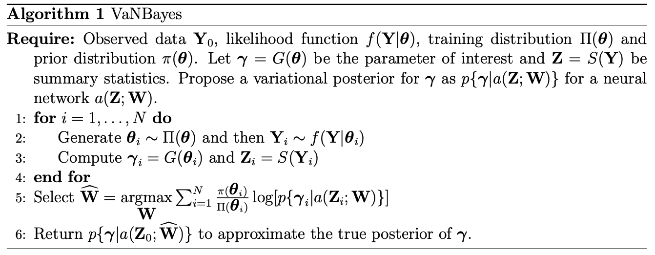
각 posterior distribution에 곱해지는 weight인 $w$는 $w_i = \pi(\boldsymbol{\theta}_i) / \Pi(\boldsymbol{\theta}_i)$로 쓸 수 있다. 여기까지 VaNBayes를 위한 사전 준비는 모두 끝났다. VaNBayes 알고리즘은 다음과 같다.

앞서 설명한 training distribution, likelihood 등이 필요하며, 우선 training distribution에서 parameter를 sampling하며 이것을 바탕으로 새로운 data $Y_i$를 generate 하며, 이것의 요약 통계량 $Z$와 parameter theta의 요약 값인 gamma를 계산한다. (1~4)

그 후 neural network의 weight인 $\boldsymbol{W}$를 조정해가며 log-posterior distribution의 likelihood가 최대가 되는 neural network weight $\widehat{\mathbf{W}}$를 구한다. (5)

최종적으로 true posterior에 근사하게 되는 neural network의 weight기반 estimated posterior를 구할 수 있다. (6) 이때 우리는 theta에 대한 posterior가 아닌 gamma에 대한 posterior를 구하는 것에 관심이 있으므로 gamma에 대한 posterior를 도출해낸다.

VaNBayes가 작동하는 이론적 이유는 논문 2.3에 잘 나와있다. true joint posterior와 marginal * neural network posterior 사이의 Kullback-Leibler divergence가 최소화되는 방향으로 neural network weight가 학습된다는 것이 주된 내용이다.

또한 실험을 통해서도 도출된 posterior가 실제에 잘 근사하는지 평가하는 과정이 있다. log score $LS = \sum_{v=1}^V \log p\{\boldsymbol{\gamma}_v \mid a(\boldsymbol{Z}_v ; \widehat{\mathbf{W}}) \}$ 를 사용하여 서로다른 data $(\boldsymbol{\gamma}_v, \boldsymbol{Z}_v)$에 대한 특정 model $a(\cdot)$의 fit을 평가한다.

2. 실험

마지막으로 VaNBayes를 사용한 다양한 실험과 결과 등에 대해 살펴보자.

2.1 Sparse linear regression

- 실험 세팅 및 순서

먼저 아래와 같은 Sparse linear regression model에서 coefficient beta를 잘 capture하는지 실험하고, 최종적으로 그 결과를 MCMC를 사용해 sampling한 것과 비교하였다.

최종 목표는 $\sigma$와 posterior inclusion probability $\text{PIP}_j = \text{Prob}(\beta_j \neq 0 \mid \mathbf{Y}) \ \text{for } j \in \{1,\dots,p\}$를 estimate하는 것이다.

$$Y_i = \beta_0 + \sum_{j=1}^p X_{ij} \beta_j + \epsilon_i$$

$\epsilon_i \overset{iid} \sim N(0, \sigma^2), i \in \{1,\dots,n\}$, 각 X들은 평균 0, 분산 1이며 $Cor(X_{ij},X_{ik})=\rho^{\lvert j-k \rvert}$인 상관관계를 가진다.

우리가 관심있는 model parameter인 $\beta$는 true 값이 $\beta_0=0, \beta_1=\beta_2=\beta_6=0.5$이며 1, 2, 6을 제외한 나머지 $\beta_j=0$ 이다. $\rho=0.5, \sigma=1$로 설정했으며 각 50개의 데이터에 대한 총 100번의 실험을 반복하였다. covariate $p$의 개수는 10개, 20개인 경우를 각각 진행하였다.

전반적인 실험의 순서는 아래와 같다.

1. 위 모델에서 data generation (100 sets)

2. summary statistic과 gamma 사용하여 neural network training

3. PIP와 sigma estimate

앞서 살펴본 VaNBayes를 위해 필요한 것이 $\gamma, Z$ 임을 알았다.

우선 $\gamma$의 경우 $\gamma_j = \mathbb{I}(\beta_j \neq 0) \in \{0,1\}, j \in \{1,\dots,p\}, \gamma_{p+1} = \sigma, \gamma_{p+1+i} =Y_{n+i}, i\in \{1,\dots,10\}$ 로 설정하였다.

그 다음 $\mathbf{Z}$를 설정한 방법에 대해 살펴보면, $(\beta_0,\dots,\beta_p)$의 least squares estimate & residual standard deviation & standard deviation of the least square estimates의 총 $p+3$의 summary statistic을 사용하였다.

또한 두 개의 hidden layer를 가지는 feed forward neural network $a_j(\mathbf{Z} ; \mathbf{W}_j)$ 를 구성하여 logistic regression model $logit\{P(\gamma_j=1 \mid \mathbf{Z})\} = a_j(\mathbf{Z} ; \mathbf{W}_j)$를 fit 하였다.

- 실험 결과

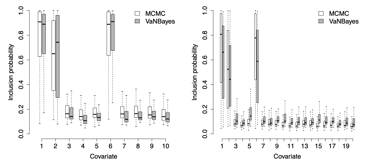
위에서 적은 내용 이외에도 neural network weight의 node수를 정하는 방법 등이 첨부되어 있으며, PIP 를 예측한 실험 결과 및 MCMC 결과와의 비교는 아래 그림과 같다.

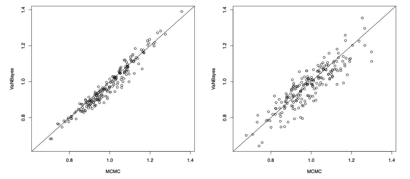
covariate의 수가 증가하는 경우에 VaNBayes가 일부 PIP를 underestimate하는 경향이 있으나 전반적으로는 MCMC와 비슷한 예측을 하는 것을 알 수 있다. 또한 아래 그림처럼 Sigma 역시 MCMC의 결과와 비슷하게 예측한 것을 알 수 있다.

2.2 Autologistic regression model

다음으로 살펴볼 실험은 autologistic regression model에서의 parameter beta의 posterior의 estimate 실험이다. 간단히 말해서 autologistic은 covariate $X_i$와 node i 의 이웃들을 고려하여 $Y_i\in \{0,1\}$의 값을 가지게 된다. 주변 데이터와의 dependency를 모델링 한 것이라고 볼 수 있겠다.

autologistic 실험에서도 앞선 실험에서 했던 것과 비슷한 세팅이 필요하다.

- 실험 세팅 및 순서

autologistic model의 full conditional distribution of one node given the others는 다음과 같다.

$$logit\{\text{Prob}(Y_i=1\mid Y_j, j \neq i)\} = logit(\kappa_i) + \phi \sum_{j\in \mathcal{N}_i} (Y_j - \kappa_j)$$

$\mathcal{N}_i$는 node i와 연결된 다른 노느들의 indices의 집합이다. 또한 $logit(\kappa_i) = \mathbf{X}_i^\top \boldsymbol{\beta}$는 covariate effect $\boldsymbol{\beta} = (\beta_1,\dots,\beta_p)$를 가지는 logistic regression probability이며 $\phi>0$은 dependence의 강도를 나타낸다.

관심있는 parameter 역시 $\boldsymbol{\beta}, \log(\phi)$이며 이들의 prior는 standard normal distribution이다. neural network를 train하기 위한 summary statistic $\mathbf{Z}$로 사용한 것은 각 $\beta_j$들의 logistic regression estimates & $\widehat{\boldsymbol{\beta}}_{GLM}$ & Geary's C statistics이다.

$\boldsymbol{\gamma}$로는 parameter를 그대로 사용하여 $\boldsymbol{\gamma}=\boldsymbol{\theta}=[\beta_1,\dots,\beta_p,\log(\phi)]$ 이다.

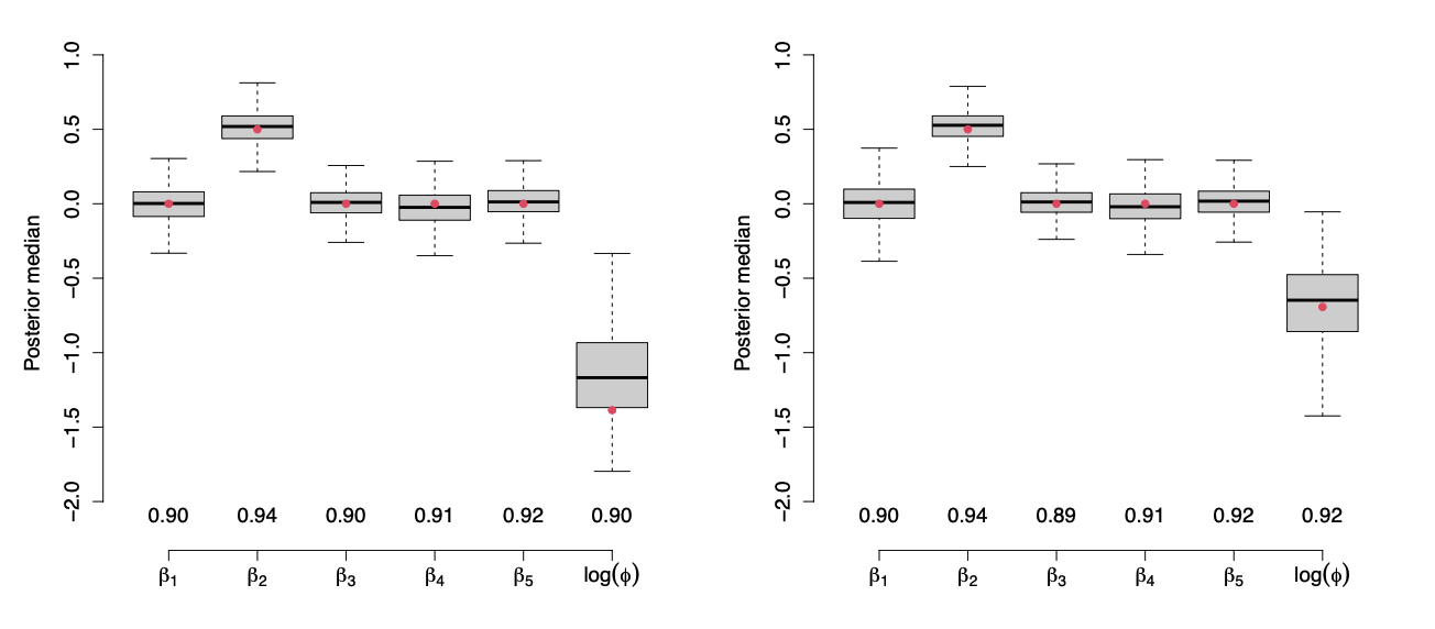
20 by 20 grid에서 400개의 data를 simulation하였고, covariate effect의 수(p) = 5로 설정하였다. 이것을 100,000번 반복하여 neural network를 train하였다. 그 결과는 아래와 같은데 dependency,$\phi$,가 작은 경우는 posterior median이 조금 벗어나있긴 하지만 다른 parameter들에 대해서는 true parameter인 red dot과 비교했을때 매우 훌륭한 예측을 한 것을 볼 수 있다.

3. 요약

지금까지 bayesian neural network를 사용하여 parameter를 estimation하는 방법에 대해 살펴보았다. 여기서 주된 내용은 parameter에 대한 direct한 estimation이 아닌 최종적으로 posterior distribution을 estimate하는 neural network를 만들었다는 점이다.

또한 parameter와 그에 기반해 생성한 data $Y$를 그대로 input하여 사용하기 보다는 차원을 축소하여 computational efficiency를 높이기 위해 summary statistic과 같은 input을 사용하였으며 Q-dimensional summary $\boldsymbol{\gamma}$에 대한 inference를 진행하였다.

알고리즘을 간략히 요약하자면 최종 목표가 observed data $\mathbf{Y}_0$의 parameter에 대한 estimation이라고 했을때, VaNBayes에서는 training distribution에서 parameter를 sampling하고, 그를 기반해서 새로운 $\mathbf{Y}_j$를 sampling한다.

그 후에 parameter와 data의 차원을 줄인 후 posterior distribution의 log-likelihood를 최대로 만드는 neural network weight $\widehat{\mathbf{W}}$를 찾는다.

Ref: Maceda, E., Hector, E. C., Lenzi, A., & Reich, B. J. (2024). A variational neural Bayes framework for inference on intractable posterior distributions. arXiv preprint arXiv:2404.10899.

1. Abstract

Spatio-temporal point process(STPP)란 시간, 공간에 따른 사건의 stochastic collection이다. 계산 복잡도를 고려하여, 기존의 시공간 통계학에서는 시간과 공간(time and space)의 conditional independence를 활용하여 distribution을 따로 구해 STPP의 solution을 도출하였다 (시간을 modeling하기 위해 Poisson process, Hawkes process 등이 사용되며 공간을 modeling하기 위해 kernel density estimator가 사용된다).

그러나 이들은 시공간을 통합하는 joint distribution을 구하지 못하는 것이 제한된 성능을 발휘할 수 밖에 없다고 생각한다 (예를 들어 지진의 발생은 이전 지진과 가까운 지역 및 시간대에 발생한다). 따라서 이를 극복하기 위해 STPP의 parameteriazaion framework를 diffusion model을 사용하여 제안한다.

Diffusion model의 input으로 spatial, temporal domain의 embedding 값을 구하여 사용하였으며, diffusion model을 통해 최종적으로 그들이 얻고자 하는 것은 hidden representation이 given 되었을 때 origial time and space를 estimate한 time and space이다.

2. Difficulties to derive spatio-temporal joint distributions

시공간의 joint distribution을 구하는 것은 아래와 같은 두가지의 이유로 쉽지만은 않다.

1. 시공간 joint distribution for STPPs는 sample space가 매우 거대하며, 이는 intractable하다. 따라서 우선 temporal density $p^*(t)$를 fitting한 후에 conditional density $p^*(s\mid t)$를 순차적으로 fitting하는 방법이 있으나, $p^*(s \mid t)$는 특정 model structure (KDEs, CNFs 등)에 제한된다.
2. 사건의 발생은 시공간 사이의 복잡한 correlation과 연관이 있다. 다양한 분야에서 발생한 사건은 그 분야에 따라 distinct한 spatio-temporal dependencies를 가진다. 따라서 대부분의 문제에 들어맞는 근본적인 시공간 dependence를 capture하는 방법이 필요하다.

따라서 이들은 새로운 parameterization framework인 Spatio-Temporal Diffusion Point Processes (DSTPP)를 제안한다. 간단히 아이디어를 설명하자면 diffusion 방법의 denoising probabilistic modeling을 활용하여 original complex distribution을 Markov chain of multiple steps로 decompose한다.

3. Spatio-temporal diffusion point processes

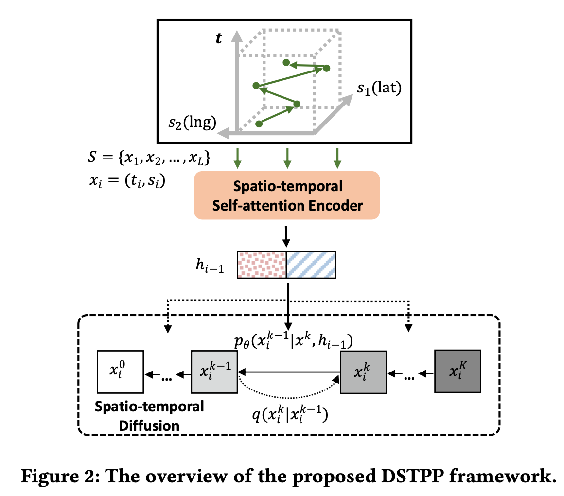
이들이 제안한 framework는 위와 같다. 크게 2개의 key module, spatio-temporal self-attention encoder와 spatio-temporal diffusion model로 구성되어 있다.

3.1 Spatio-temporal Encoder

이 단계는 spatio-temporal data를 embedding하고, hidden representation을 추출하는 과정이다. 시공간 데이터를 input하면 embedding layer와 attention layer를 거쳐 hidden representation을 반환한다. 저자들은 이 과정을 Encoding으로 생각하여  Encoder라고 표현한 듯 하다.

우선 시간을 embedding하는 방식은 아래와 같다. $M$은 embedding dimension이며 따라서 $e_t$가 temporal embedding을 나타낸다.

$$[e_t]_j = \begin{cases} \cos(t/10000^{\frac{j-1}{M}}) \text{ if j is odd} \\ \sin(t/10000^{\frac{j-1}{M}}) \text{ if j is even} \end{cases}$$

공간은 다음과 같이 embedding한다. $W_e$는 학습가능한 parameter를 포함하며 공간이 continuous domain인 경우 (like 좌표 데이터)와 discrete domain인 경우 (like lattice data)에 모두 사용 가능하다.

$$e_s = W_e s$$

또한 위 두개의 embedding 결과를 더하여 spatio-temporal embedding $e_{st}$를 정의할 수 있다.

결과적으로, 시공간 데이터 $S = \{(t_i, s_i)\}_{i=1}^L$에 대해 시공간 embedding $E_{st} = \{e_{st,1},\dots,e_{st,L}\}$, 시간 embedding $E_s = \{e_{t,1}, \dots, e_{t,L}\}$, 그리고 공간 embedding $E_s = \{e_{s,1}, \dots, e_{s,L}\}$을 얻을 수 있다.

그 다음 목표는 이 3가지의 embedding을 활용하여 서로다른 시공간마다의 characteristic을 capture하는 것이다. 따라서 논문의 (7), (8)번 수식을 통해 embedding vector들의 연산을 하고 최종적으로 spatial, temporal, and spatio-temporal 각각에 대한 hidden representation에 대해 얻을 수 있게 된다.

3.2 Spatio-temporal Diffusion and Denoising Processes

위에서 hidden representation, $h_{i-1}$을 얻은 그 다음의 목표는 hidden representation을 conditioning하여 미래 event에 대한 spatio-temporal joint distribution의 model을 학습하는 것이다. 그리고 여기에 diffusion model을 활용하였다.

이들은 space와 time에 각각 noise를 더하고 이를 복원하는 식으로 diffusion process와 reverse process를 진행하였다. 각 event $x_i =(\tau_i, s_i), \text{ (where } \tau_i \text{ denotes the time interval since the last event) }$에 대해 diffusion process modeling을 위해 K번의 diffusion process를 거친 Markov process $(x_i^0, x_i^1, \dots, x_i^K)$를 적용하였다. 각 diffusion step에 Guassian noise를 더해가는 과정을 다음과 같이 쓸 수 있다.

$$q_{st}(x_i^k \mid x_i^{k-1}) = (q(\tau_i^k \mid \tau_i^{k-1}),q(s_i^k \mid s_i^{k-1})), \\q(x^k \mid x^{k-1}) = N(x_k ; \sqrt{1-\beta_k}x^k, \beta_k \mathbf{I})$$

반면 noise를 제거해가며 원본 data $x_i = (\tau_i, s_i)$를 복원하는 과정, reverse process는 hidden representation을 condition으로 아래의 분포를 얻는 과정이다.

$$p_\theta(x_i^{k-1} \mid x_i^k, h_{i-1}) = p_\theta(\tau_i^{k-1} \mid \tau_i^k, s_i^k, h_{i-1})p_\theta(s_i^{k-1} \mid \tau_i^k, s_i^k, h_{i-1})$$

이전 event까지의 hidden representation을 given하여 다음 event의 시간과 공간의 joint distribution을 서로 conditionally independent하게 만들 수 있다는 의미인 듯 하다.

따라서 위 방법을 사용하여 diffusion model을 train하고, trained model을 사용하여 real data $(\tau_i^0, s_i^0)$에 대한 prediction값을 얻을 수 있다. 또한 이 prediction에서 중요한 것은 co-attention denoising network를 사용했다는 점이다. 이는 spatial과 temporal domain의 상호의존성을 capture하기 위함이며 3.4에 자세히 나와있다.

4. Experiments

이들은 real dataset과 synthetic dataset에서 다양한 실험을 진행하였다. 그 중 몇가지의 과정과 결과만 살펴보자. 이들은 Earthquakes, COVID-19 등의 real datasetrhk HawkewGMM의 synthetic dataset을 사용하였으며 이들이 구한 model vs 기존의 baseline model에서의 모델 성능을 두가지 측면으로 비교하였다. 첫번째는 space와 time각각의 negative log-likelihood를 구하여 비교하는 것이고, 두번째는 time은 RMSE, spatial location은 Euclidean distance를 계산하여 비교한 것이다.

결과를 살펴보면 이들의 model DSTPP는 모든 dataset에서 가장 뛰어나거나 두번째로 뛰어난 성능을 보였다. 기존의 NSTPP와 같은 conditional distribution을 사용하여 시공간의 distribution을 구하는 방식은 spatial 측면에서는 시간과 공간의 independence를 가정하고 modeling한 결과보다는 뛰어났지만, temporal 측면에서는 temporal modeling만 사용한 다른 방식들에 비해 아주 뛰어난 성능을 보이지는 않았다. 이러한 방법도 시공간의 joint distribution을 구한 것은 동일하지만 temporal domain은 잘 학습하지 못함을 보여주는 결과였다.

References:

Yuan, Y., Ding, J., Shao, C., Jin, D., & Li, Y. (2023, August). Spatio-temporal diffusion point processes. In Proceedings of the 29th ACM SIGKDD Conference on Knowledge Discovery and Data Mining (pp. 3173-3184).

0. Overview

공간통계학에서 우리는 통계적 Modeling을 위해 보통 stationary 가정을 한다. 이는 간단히 말해서 특정 지점사이의 거리가 같다면, 공분산이 같음을 의미한다 (분산이 특정 지점 사이의 거리차이에 depend). 그러나 단순히 홍대입구역부터 신촌역까지의 거리와, 홍대입구역부터 합정역 까지의 거리의 같다는 사실이 각 지점의 특성이 같다는 것을 의미하지는 않는다. 예를 들어 강수량과 같은 수치는 단순한 거리 차이보다 각 지점의 온도나 고도 등에 더 많은 영향을 받는다.

따라서 이러한 공간적 특성을 반영하기 위해 modeling시에 nonstationary 가정을 해야하지만 이는 분석이 쉽지 않다. 이들은 Convolutional neural networks (CNN)을 사용하여 공분산을 modeling하였는데 이에 대해 살펴보도록 하겠다. 또한 CNN을 사용하기 위해 좌표 data를 어떻게 CNN의 input으로 변환하였는지를 중점적으로 살펴보도록 하겠다.

1. Methods

기존에 존재하는 nonstationary covariance modeling 방법은 1) spatial deformation method, 2) process convolution approach 등이다. 구체적인 설명은 생략하고 2)에서는 matern covariance의 closed form을 구할 수 있는데, 지역의 수가 많아질수록 계산해야하는 matrix의 크기가 커지며 따라서 추정하기 힘들다는 단점이 있다. 따라서 구역(subregion)을 나누어 local stationary를 가정하는 방법들이 후에 제안되었는데 이러한 방법은 subregion을 나누는 것이 주관적이라는 단점이 존재한다.

이들은 spatial data를 incomplete image로 여기고(image는 특정 image size에서 모든 점들이 관측되어 RGB의 값을 가지지만, spatial data는 관측이 되지 않는 지점이 존재하므로 이를 관측되지 않은 RGB로 생각) CNN을 사용하여 주관적으로 subregion을 나누는 기존의 방법을 data-driven 방법을 제안함으로서 (조금 더 객관적) 개선하고자 한다. 

2. CNN model

2.1  CNN architecture

CNN model을 사용한 이유는 위에서 언급한 것과 같이 stationary 와 nonstationary region을 구분하기 위함이다. 따라서 100 by 100 크기의 input에 따라 구역이 nonstationary할 확률을 output한다. 따라서 분류문제로 생각하여 확률이 0.5보다 크거나 같으면 저자는 nonstationary 구역으로 생각하고 그렇지 않으면 stationary 구역으로 생각하여 모델을 학습하고 사용한다.

구체적으로 이들이 사용한 CNN 구조는 위와 같다. 우선 100 by 100 size의 input data를 3 by 3의 kernel 32개를 사용하여 feature를 extract하는 convolution layer를 거친다. 그 후 flatten layer로 이를 vector로 펼치고 마지막으로 FC layer에서 두 단계의 non-linear transformation을 거쳐 최종적으로 nonstationary region일 확률을 나타낸다.

2.2 Data pre-processing

그러나 문제점이 존재하는데 CNN을 사용하기 위해서 100 by 100 size의 input 형태로 data를 변환해야하지만 현실 세계의 많은 데이터는 100 by 100 grid에 맞게 균일하게 위치하지 않는다는 것이다. 따라서 이들은 3단계의 전처리 과정을 거쳐 100 by 100 size의 input형태를 만들어내며 구체적인 설명은 다음과 같다. 

• Splitting: divide observed region $[0,1]^2$ to 100 by 100 subregions (denote each subregion as $D_{i,j}$)
• Averaging: $D_{i,j}$에 속하는 observation의 개수를 $N_{i,j}$, $D_{i,j}$에 속하는 observation들의 평균을 $\bar{Z}(i,j)$라고 하여 아래와 같이 계산한다.

$$\bar{Z}(i,j) = \begin{cases} \frac{1}{N_{i,j}} \sum_{k:s_k \in D_{i,j}} Z(s_k), \quad N_{i,j}>0 \\ \bar{Z}(u,v), \ \text{where }(u,v) = argmin_{u,v}\{(i-u)^2 + (j-v)^2 : N_{u,v}>0\}, \quad N_{i,j}=0 \end{cases}$$

• Scaling: 위에서 얻은 $\bar{Z}(i,j) \in [0,1]$의 minimum을 m, maximum을 M이라고 하자. 아래와 같이 scaling을 한다.

$$\tilde{Z}(i,j) = \begin{cases} (\bar{Z}(i,j) - m) / (M-m), \ \ m \neq M; \\ 0.5, \quad \quad m=M \end{cases}$$

위 과정을 요약하자면, $[0,1]^2$의 좌표를 100 by 100의 subregion으로 나눈 후, 각 subregion에 속하는 점들의 GRF값의 평균을 취한 다음 minmax scaling을 한다. 결과적으로 우리가 원하는 100 by 100 size의 input 형태를 갖추게 된다. (그런데 location 좌표 $s_k$를 subregion $D_{i,j}$에 어떻게 mapping하는 지는 나와있지 않다)

2.3 Subregion selection

이제 남은 것은 train한 CNN과 전처리한 data를 사용하여 stationary한 지역과 nonstationary한 지역을 나누는 것이다. 이를 위해서 subregion을 나누어야 한다 (input size를 100 by 100으로 나누기 위해 2.2에서 정의한 subregion과 다름). 이들이 제안한 방법을 정리하면 다음과 같다.

1.  좌표 $S = \{s_1,\dots,s_n\}$에서 K개의 random한 point $A = \{a_1, \dots, a_K\}$를 선택한다.
2. 그 후 distance vector $E = \{ \lVert s_i - a_k \rVert^2: a_k \in A\}$를 계산한다. distance vector는 특정 point $s_i$에서 random하게 선택된 K개의 point $a_k$까지의 거리이며 따라서 성분이 K개이다.
3. 특정 점 $s_i$가 $a_j$와 거리가 가장 최소라면, subregion $R_j$에 $(s_i, Z(s_i))$를 할당한다.
4. 각 subregion$\{R_k\}_1^{K}$마다 2.1의 CNN 구조를 사용하여 nonstationary probability를 구한다 (let this $p_k, k=1,\cdots,K$).
5. $P = \sum_{k=1}^K p_k$를 구한 후 iteration을 반복하여 최소가 되는 $P$를 찾고 그때의 subregion에 속하는 점들의 centre를 반환한다 (각 iteration마다 선택되는 점의 집합 $A$가 다르므로 $P$도 달라진다).

요약하자면 몇 개의 subregion으로 나눌 것인지만 선택하면, 우리가 가진 데이터들이 어느 subregion에 속하는지 알 수 있는 알고리즘이다. 다만 최적의 subregion수 K를 선택하는 방법이 없다는 것은 조금 아쉽다.

3. Simulation

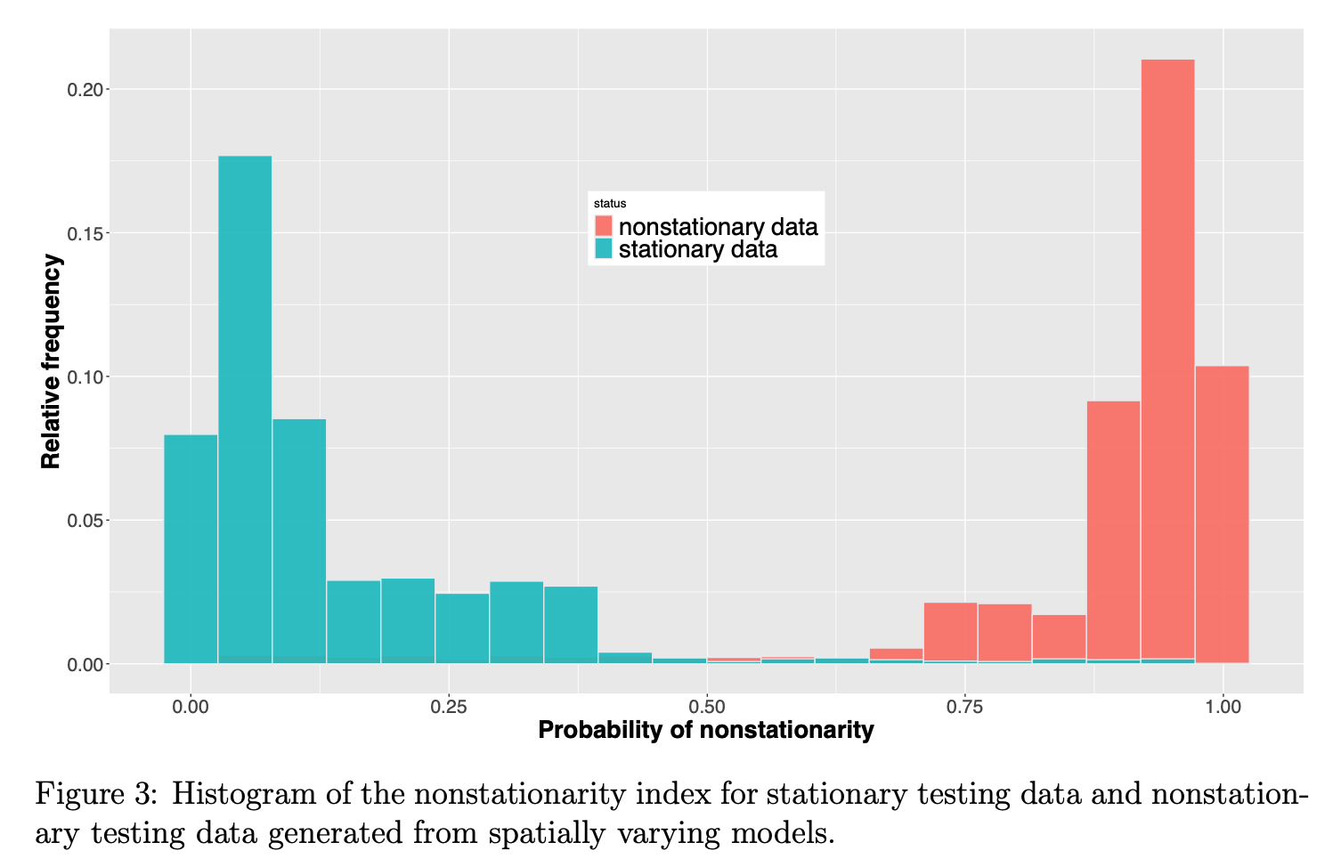
이들은 두 종류의 simulation을 하였다. 간략히 설명하자면 첫번째 실험은 stationary or nonstationary여부를 CNN이 잘 구분하는가에 관한 실험이다. 과정은 우선 stationary, nonstationary dataset을 각각 16000개 generate 한 후 80%의 sample을 활용해 CNN을 train한다. 구체적인 data generation과정은 생략하고, 남은 20%의 데이터를 활용해 test한 결과는 아래와 같다.

간혹 stationary data인 것을 nonstationary로 판단하는 경우(and 그 반대)가 있었지만 대체로 정확한 classification을 한 것을 알 수 있다.

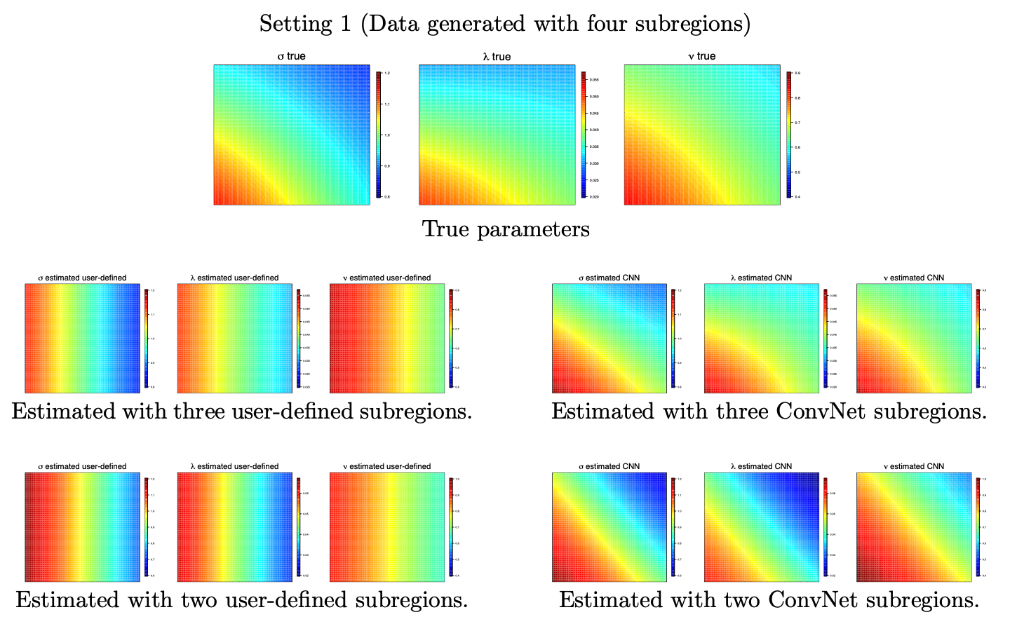
두번째 실험은 $[0,1]^2$ domain에서 4개의 기준 점(anchor locations)을 기준으로 하여 4가지의 서로 다른 nonstationary parameter를 가지는 subregion에서 10,000개의 nonstationary data를 생성한다. 그 후 2&3개의 subregion을 가지도록 CNN을 학습한다. 여기서 실제로 나눈 subregion과 비슷하게 구역이 나뉘는지 check할 수 있으며, ExaGeoStat package를 사용하여 nonstationary data의 parameter또한 추정할 수 있는데, CNN model을 사용하여 추정한 parameter의 MSE vs. 기존 방식으로 subregion을 나눈 후 추정한 parameter의 MSE를 비교하였다.

추정 결과를 간단히 살펴보자면 CNN으로 subregion을 나눈 후 parameter를 추정하면 user-defined subregion보다 실제 parameter를 더 잘 추정하는 것을 알 수 있다.

4. 요약

이 논문은 공간통계학에서 stationary 가정이 위배되는 많은 상황이 있다는 것에서 출발하여, 기존의 local stationary 방법이 주관적인 선택에 의해 subregion을 만드는 것에 문제를 제기하고, CNN을 통해 subregion을 만드는 방법을 개선하고자 하였다. Stationary 가정을 local하게 하되, 객관적인 방법으로 subregion을 만든 후 subregion내의 point 사이의 local stationary를 가정하여 분석하는 방안을 제시한 것이다.

References:

Nag, P., Hong, Y., Abdulah, S., Qadir, G. A., Genton, M. G., & Sun, Y. (2023). Efficient Large-scale Nonstationary Spatial Covariance Function Estimation Using Convolutional Neural Networks. arXiv preprint arXiv:2306.11487.

0. Preliminary

ETAS point process

시작에 앞서 논문을 이해하기 위해 ETAS point process에 대한 사전지식이 필요하다. Epidcmie-Type Aftershock Sequence (ETAS) model이란 날짜, 시간, 위도, 경도, 지진의 진도 등을 사용하여 지진의 발생을 modeling하는 과정이다.

수식적인 설명을 덧붙이면 이는 conditional intensity $\lambda(t, x, y, m\mid H_t)$를 사용한 point process 이다.

이 intensity function의 notation들을 조금 더 자세히 살펴보자면, $(x, y)$는 2차원 좌표이며 $m, t$는 진도와 시간이다. 또한 $H_t$는 $t$ 시점까지의 process들의 history이며 $\Big(H_t = (t_i, x_i, y_i, m_i) : t_i \le t \Big)$, 따라서 intensity function은 t시점 이전까지의 event들이 given되었을 때, 시간 $t$, 좌표 $(x,y)$, 진도 $m$인 이벤트가 발생할 expected rate라고 해석할 수 있다.

또한 이는 Hawkes' point process의 special case인데, conditional intensity function을 아래와 같이 decompose 할 수 있다.

$$\lambda_{\beta, \Theta}(t, x,y,m\mid H_t) = \nu_\beta(m)\lambda_\Theta(t,x,y \mid H_t)$$

여기서 $\nu_\beta (m)$은 magnitude m 의 pdf with unknown parameter $\beta >0$이다. 오른쪽 $\lambda$ 함수는 다음과 같이 decompose가 가능하다.

$$\lambda_\Theta(t,x,y\mid H_t) = \tilde{u}(x,y) + \sum_{t_i < t} \kappa_{A,\alpha}(m_i) g_{c,p}(t-t_i) f_{D,\gamma,q}(x-x_i, y-y_i;m_i)$$

$\tilde{u} (x,y)$: $\mu >0$을 모수로 가지는 background seismicity (지진활동도) rate를 나타낸다.

$\kappa_{A,\alpha}(m_i)$: 진도가 $m_i$로 발생하는 지진의 기대 발생 횟수이다.

$g_{c,p}(t-t_i)$: 지진 발생 시간에 대한 probability density function이다.

$f_{D, \gamma, q}(x-x_i, y-y_i ; m_i)$: 지진이 발생하는 좌표에 대한 probability density function이다. 이때 진도는 $m_i$이다.

Interpretable Deep Generative Spatio-Temporal Point Processes

1. Goal

위 논문에서는 Neural Embedding Spatio-Temporal (NEST) point process를 제안한다. 위에서 언급한 지진의 모델링에 많이 사용하던 ETAS는 kernel function이 location에 상관 없이 homogeneous한 성질이 있어서 model fitting이 용이하였지만, 이러한 고전적인 모델들은 conditional intensity의 parameter 값에 의존할 수 밖에 없다는 단점 또한 존재한다.

따라서 NEST model은 복잡한 spatial dependence를 더 잘 capture하고, 해석이 가능하며, computation에도 장점이 있다.

(intensity function이란 시간, 공간에 따른 사건 발생률의 함수이며, conditional intensity function은 과거 사건의 발생을 고려한다.)

2. Method

이들은 continuous-time and continuous space point process model인 NEST model을 제안한다. NEST model에서는 intensity function으로 neural network를 사용하게 되는데, parameter에 의존하는 기존의 방법들과는 달리 이들은 neural network를 사용함으로 model의 interpretability를 유지하며 flexibility를 줄 수 있다고 주장한다.

구체적으로 이들은 다음과 같은 conditional intensity function을 제안한다.

$$\lambda^*(t,s) = \lambda_0 + \sum_{j:t_j<t}\nu (t,t_j,s,s_j)$$

$\nu$는 과거 사건 $\mathcal{H}_t$의 영향을 capture하는 kernel function이며, 여기서는 standard Gaussian diffusion kernel 형태의 커널을 사용했다. (사건 간의 시공간적 dependency를 결정하는 함수)

kernel function의 구체적인 형태는 다음과 같다.

$$\nu(t,t^\prime, s, s^\prime) = \sum_{k=1}^K \phi_{s^\prime}^{(k)} \cdot g(t,t^\prime, s, s^\prime \mid \Sigma_{s^\prime}^{(k)} , \mu_{s^\prime} ^{(k)}), \quad \forall t^\prime < t, s \in \mathcal{S}$$

term들을 조금 더 자세히 살펴보자면,

$\{\mu_{s^\prime}^{(k)}, \Sigma_{s^\prime}^{(k)}\}$:  mean and covariance matrix parameters

$K$:  Gaussian mixture의 component 수를 결정하는 hyper-parameter

$\phi_{s^\prime}^{(k)}:\mathcal{S} \rightarrow \mathbb{R}$:  $\sum_{k=1}^K \phi_{s^\prime}^{(k)}=1, \forall s^\prime \in \mathcal{S}$를 만족하는 k-th Gaussian component의 weight

$g(\cdot)$ 함수의 구체적인 형태는 다음과 같다.

$$g(t, t^\prime, s, s^\prime) = \frac{Ce^{-\beta(t-t^\prime)}}{2\pi \sqrt{\lvert \Sigma_{s^\prime} \rvert}(t-t^\prime)}\cdot \exp \Big\{ - \frac{(s-s^\prime - \mu_{s^\prime})^\top \Sigma_{s^\prime}^{-1}(s - s^\prime - \mu_{s^\prime})}{2(t-t^\prime)} \Big\}$$

$\beta>0$가 커질수록 위 함수의 값이 빠르게 감소하므로, 이는 temporal decay rate를 조절하는 parameter이며, $C>0$은 constant로 값의 magnitude를 조절한다.

$\mu_s = [\mu_x(s), \mu_y(s)]^\top, \Sigma_s$는 diffusion kernel의 mean and covariance parameters를 의미하며, Ganssian component들의 shift, rotation, shape을 결정하는 parameter이다.($\Sigma$는 positive semi-definite matrix이다).

3. Conclusion

결과적으로 저자들은 자신들의 방법 (NEST)가 기존의 ETAS 방법을 사용했을 때보다 spatial dependency를 더 잘 capture한다고 주장한다. 또한 model parameter 추정에서 neural network를 사용한 것 같은데, model의 기조는 Gaussian diffusion kernel이므로 parameter값에 대한 해석이 가능하기 때문에 interpretable이라는 단어를 논문 제목에 붙인 것 같다. 구체적인 실험 결과 및 수식은 본문의 Chapter 4와 Appendix에서 확인 가능하다.

References:

Zhu, S., Li, S., Peng, Z., & Xie, Y. (2020). Interpretable deep generative spatio-temporal point processes. In AI for Earth Sciences Workshop at the 34th Conference on Neural Information Processing Systems (NeurIPS 2020), online, Dec(pp. 6-12).

Ogata, Y. (1998). Space-time point-process models for earthquake occurrences. Annals of the Institute of Statistical Mathematics, 50, 379-402.

Let's have some statistical inference using functional data.

Before we move on, assume that $X_1,X_2,X_3,\dots$ are i.i.d sample of random functions from $\mathcal{H}=L^2[0,1]$ with $E\lVert X_n \rVert ^2 < \infty$. And $\mu$ and $C$ indicate mean and covariance respectively.

Recall

Recall that sample version of mean and covariance are as follows:

$$\hat{\mu}(t) = \frac{1}{N} \sum_{n=1}^N X_n(t), \quad \hat{c}(t,s) = \frac{1}{N} \sum_{n=1}^N \Big(X_n(t)-\hat{\mu}(t)\Big)\Big(X_n(s) - \hat{\mu}(s)\Big)$$

And also note that we can express the sample covariance operator as follows:

$$\hat{C}(x) = \frac{1}{N}\sum_{n=1}^N \langle X_n-\hat{\mu},x \rangle (X_n - \hat{\mu}) \quad \text{or} \\ \hat{C} = \frac{1}{N} \sum_{n=1}^N (X_n - \hat{\mu}) \otimes (X_n - \hat{\mu})$$

And there is a simple lemma:

If $X, Y\in \mathcal{H}$ are independent then
$$E \langle X, Y \rangle = \langle \mu_x, \mu_y \rangle$$

Proof is not that difficult.

Proof)

$$E \langle X, Y \rangle = E[ \int X(t) Y(t) dt] = \int E[X(t)] E[Y(t)] dt = \langle \mu_x, \mu_y \rangle$$

Convergence rate of sample mean

We can show that

$$E \lVert \hat{\mu} - \mu \rVert ^2 = O(N^{-1})$$

It implies the difference between true mean $(\mu)$ and estimated mean $(\hat{\mu})$ depends on our sample size $N$ and the convergence rate is $1/N$.

Proof)
$$\begin{align} E \lVert \hat{\mu}-\mu \rVert ^2 &= E \langle \frac{1}{N}\sum X_n-\mu, \frac{1}{N} \sum X_n - \mu \rangle \\ & = \frac{1}{N^2} \sum_n E \langle X_n - \mu, X_n - \mu \rangle \begin{cases} = 0, & \text{if } n\neq m \newline = \frac{1}{N} E \lVert X_1 - \mu \rVert ^2, & \text {if } n=m \end{cases} \end{align}$$
Thus we need to consider only the case of $n=m$.
Then, the final result can be written as $$N^{-1} E \lVert X_1 - \mu \rVert ^2 = O(N^{-1})$$
which completes the proof.

Upper bound for sample covariance

If $E\lVert X_n \rVert ^4 < \infty$, then we have upper bound for sample covariance as follows:

$$E\lVert \widehat{C} \rVert _{\mathcal{S}}^2 \le E \lVert X_1 \rVert ^4 \quad \text{and} \quad E \lVert \widehat{C}-C \rVert _{\mathcal{S}}^2 \le \frac{1}{N} E \lVert X_n \rVert ^4. $$

Proof will be skipped.

Hypothesis test

Using functional data, we can make hypothesis test. Our primary goal is to evaluate hypotheses like

$$H_0: E[X_n]=\mu=\mu_0 \quad \text{vs} \quad H_a:\mu\neq \mu_0$$

But the problem is there is no best way to solve this problem like scalar case. It may mean we have to approximate this problem.

Consider the multivariate case first and suppose that $X_1,\dots ,X_n$ are i.i.d random vectors in $\mathbb{R}^d$ with mean $\mu$ and covariance matrix $\boldsymbol{\Sigma}$ as before. The conventional way to test $\mu=\mu_0$ is to use Hotelling's $T^2$ test:

Hotteling's T:
$$T^2 = N(\bar{X} - \mu_0)^\top \boldsymbol{\Sigma}^{-1}(\bar{X} - \mu_0)$$

Then, $T^2 \sim \chi^2_p$ under $H_0$ while $T^2 \overset{\mathcal{P}}{\longrightarrow}\infty$ under $H_a$. But we set $X_i$ to random vector, not random function. Thus we need functional version.

In functional problems, it is hard to define inverse of $C$. General way to solve this is to use the KL expansion and asymptotic property learned earlier. Under $H_0$, we know the below asymptotic convergence from the KL expansion.

$$ \langle \sqrt{N}(\hat{\mu}-\mu), v_i \rangle \overset{\mathcal{D}}{\longrightarrow} \mathcal{N}(0,\lambda_i)$$

And it is asymptotically independent. With this property, there are several approach to make hypothesis test.

1. FPCA approach

First one is to use FPCA testing only first few principal component directions.

FPCA approach:
$$T^2_{PC} = \sum_{i=1}^p \frac{N\langle \hat{\mu} - \mu_0, \hat{v_i} \rangle^2}{\hat{\lambda_i}}$$

And we have $T^2_{pc} \overset{\mathcal{D}}{\longrightarrow}\chi ^2(p)$ under $H_0$ while $T^2_{pc} \overset{\mathcal{P}}{\longrightarrow}\infty$ as long as $\langle \mu-\mu_0, v_i \rangle \neq 0$.

But it has some weakness that it is very sensitive to the choice of p.

2. Norm approach

Second approach is Norm approach. It is full version of FPCA thus it test all of the FPC directions.

Norm approach:
$$T^2_{norm} = N \lVert \hat{\mu} - \mu_0 \rVert^2 = \sum_{i=1}^\infty N \langle \hat{\mu}-\mu_0,\hat{v_i} \rangle^2$$

Under $H_0, T^2_{norm} \overset{\mathcal{D}}{\longrightarrow} \sum_{i=1}^\infty \lambda_i \chi_i^2(1)$ while under $H_A, T^2_{norm} \overset{\mathcal{P}}{\longrightarrow} \infty$.

It has advantage that does not need to choose p. Althogh this approach uses all the FPC components, but it is not always better than PC approach, it can be better or not.

3. Choi Test

Thire method is Choi Test. It is the intermediate method between FPCA and norm approach.

Choi Test:
$$T^2_{Choi} = \sum_{i=1}^p \frac{N \langle \hat{\mu}-\mu_0, \hat{v}_i \rangle ^2}{\hat{\lambda}^{1/2}_i}$$

Under $H_0, T^2_{Choi} \overset{\mathcal{D}}{\longrightarrow} \sum_{i=1}^\infty \lambda_i ^{1/2} \chi_i^2(1)$ while under $H_A, T^2_{Choi} \overset{\mathcal{P}}{\longrightarrow} \infty$.

Confidence Band

Before we move on to the last method, there's one introduciton: Confidence Bands. In this band, our goal is to find function $r(t)$ such that

$$P\Big( r(t) \le \hat{\mu}(t) - \mu(t) \le r(t) \Big) \ge 1-\alpha$$

4. Boostrap approach

The last one is bootstrap approach. It is a simulation method that generate new samples from estimated distribution and with these new samples we make new estimated distribution.

In this approach, our goal is to generate $X_{nb}$ for $n=1,\dots,N$ and $b=1,\dots,B$. And each $X_{nb}$ is generated as follows:

$$X_{nb}(t) = \hat{\mu}(t) - \epsilon_{nb}(t)$$

And to make a connection with confidence band above, we will form a band as

$$\hat{\mu}(t) \pm \sqrt{\widehat{C}}(t,t)c_{1-\alpha}$$

And use bootstrap samples to approximate $c_{1-\alpha}$.

The bootstrap statistic is

$$D_b = \sup \frac{\lvert \hat{\mu}(t) - \hat{\mu}_b(t)\rvert}{\sqrt{\widehat{C}(t,t)}}$$

Then we take $c_{1-\alpha}$ as the $1-\alpha$ quantile of the $D_b$.